Decision trees are versatile machine learning algorithms that can perform both classification and regression tasks, and even multioutput tasks. It works by recursively partitioning the data into subsets based on statements of features, making decisions whether or not the statement is True or False.
Important notes to remember
Handle both numerical and categorical data.
Do not require feature scaling.
The algorithm selects the best feature at each decision point, aiming to maximize information gain (for classification) or variance reduction (for regression). Decision trees are interpretable, easy to visualize, and can handle both numerical and categorical data. However, they may be prone to overfitting, which can be addressed using techniques like pruning.
Ensemble methods, such as Random Forests and Gradient Boosting, often use multiple decision trees to enhance predictive performance and address the limitations of individual trees.
Decision Tree is white box model which is interpretable ML, vs Random Forest, Neural Networks is black box model (not easy to interpret).
Some DT algorithm:
ID3, C4.5 (Information Gain/ Information Gain Ratio)
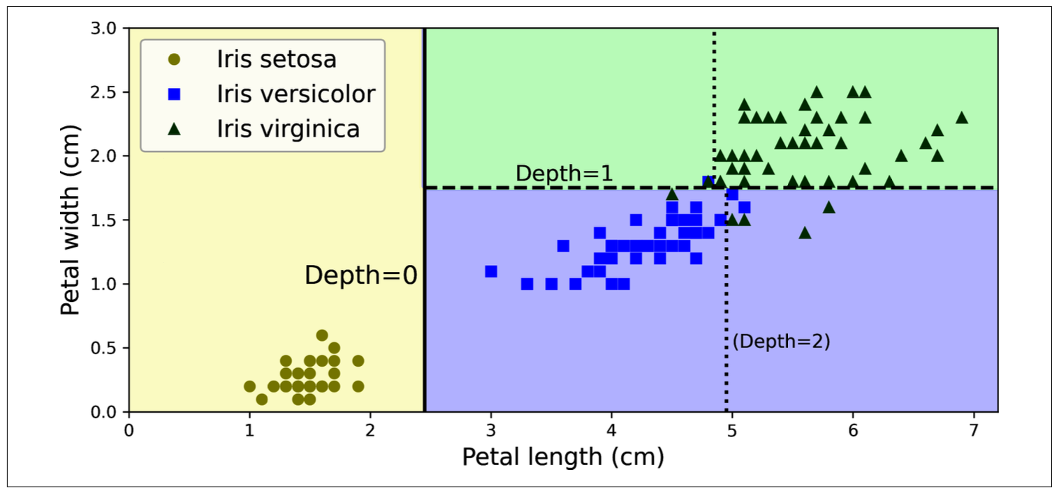
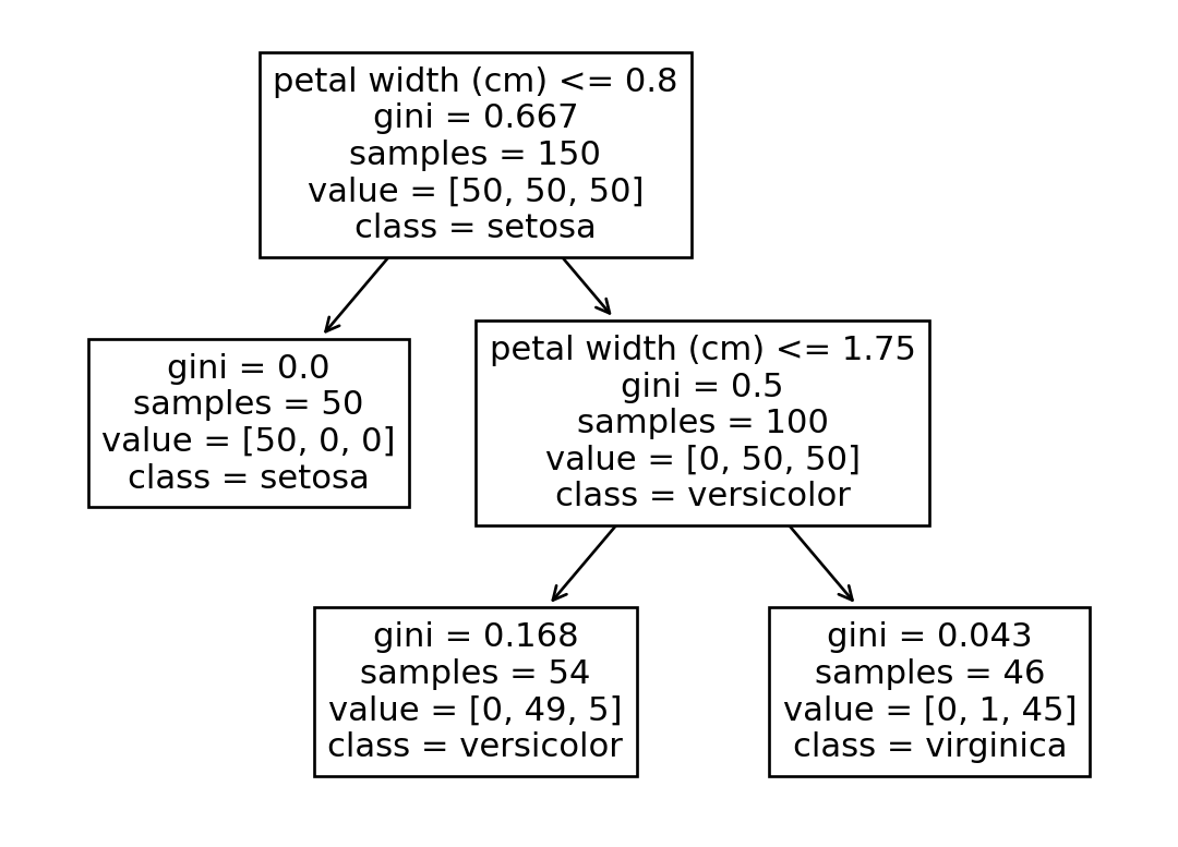
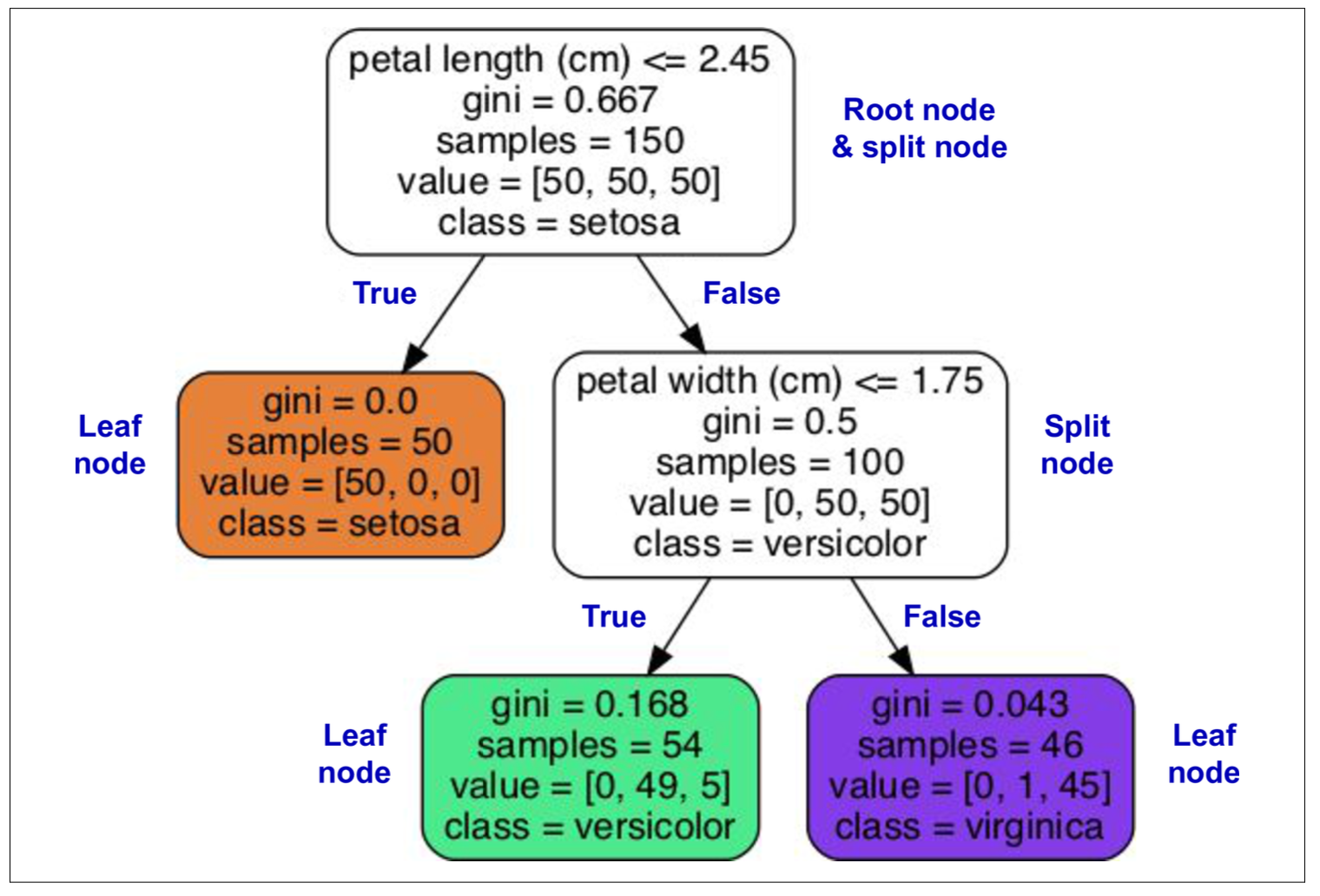
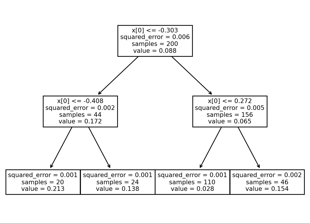
Figure fig-decision-tree, in a node:
- Samples: count instances in that node
- Value: count instances of each class
- Gini (Gini impurity): a measurement, measure a node is pure (0) or not (-> 1) \[G_{i}=1-\sum_{k=1}^{n}p_{i,k}^{2}\]
Gi: Gini impurity of node i\
pi,k: probability of `class k instances` in total instances in node `i`
CART split training set recursively until: purest, max_depth, min_samples_split, min_samples_leaf, min_weight_fraction_leaf, and max_leaf_nodes.
Find optimal tree is NP-complete problem, O(exp(m)) => Have to find ‘resonably good’ solution when training a decision tree
But making predictions is just O(log2(m))
NP-complete problem
P is the set of problems that can be solved in polynomial time (i.e., a polynomial of the dataset > size). NP is the set of problems whose solutions can be verified in polynomial time. An NP-hard problem is a problem that can be reduced to a known NP-hard problem in polynomial time. An NP-complete problem is both NP and NP-hard. A major open mathematical question is whether or not P = NP. If P ≠ NP (which seems likely), then no polynomial algorithm will ever be found for any NP-complete problem (except perhaps one day on a quantum computer).
9.1 Regularization
Parametric model (Linear Regression): predetermined parameters => degree of freedom is limited => reducing the risk of overfitting
Non-parametric model: parameters not determined prior to training => go freely => overfitting => regularization
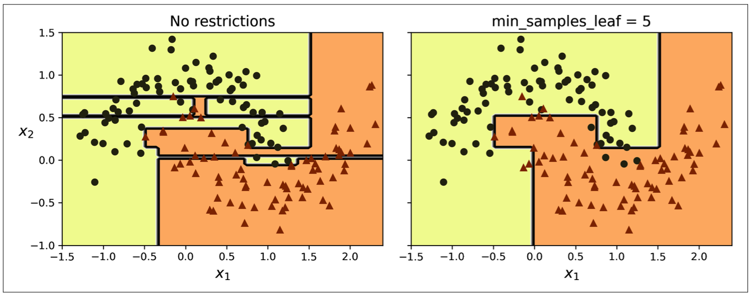
Increasing min_* hyperparameters or reducing max_* hyperparameters will regularize the model:
Figure 9.3: Decision boudaries of unregularized tree (left) and regularized tree (right)
Pruning Trees
Pruning: deleting unnecessary nodes
Algorithms work by first training the decision tree without restrictions, then pruning (deleting) unnecessary nodes. A node whose children are all leaf nodes is considered unnecessary if the purity improvement it provides is not statistically significant. Standard statistical tests, such as the χ2 test (chi-squared test), are used to estimate the probability that the improvement is purely the result of chance (which is called the null hypothesis). If this probability, called the p-value, is higher than a given threshold (typically 5%, controlled by a hyperparameter), then the node is considered unnecessary and its children are deleted. The pruning continues until all unnecessary nodes have been pruned.
There are 3 types of Pruning Trees
Pre-Tuning
Post-Tuning
Combines
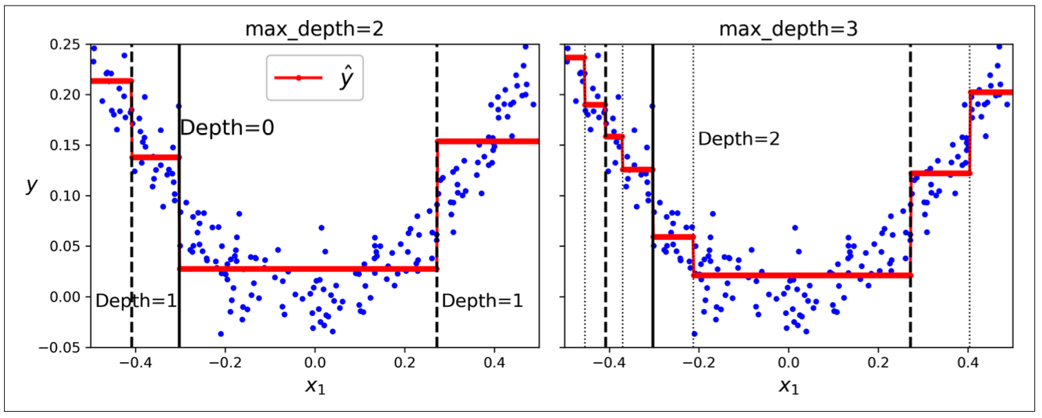
9.2 Regression
DecisionTreeRegressor splits each region in a way that makes most training instances as close as possible to that predicted value (average of instances in the region)
CART cost function for regression: \[
J_{k, t_k} = \frac{m_{left}}{m} MSE_{left} + \frac{m_{right}}{m} MSE_{right}
\]
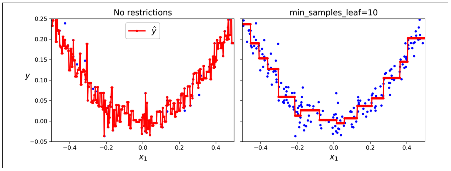
Figure 9.5: Unregularized tree (left) and regularized tree (right
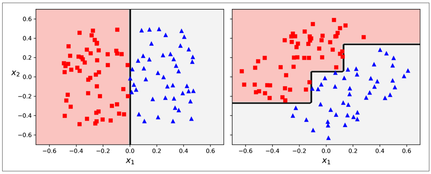
9.3 Limitations of Decision Tree
Decision tree tends to make orthogonal decision boudaries. => Sensitive to the data’s orientation.
Figure 9.6: Decision tree is sensitive to data’s orientation
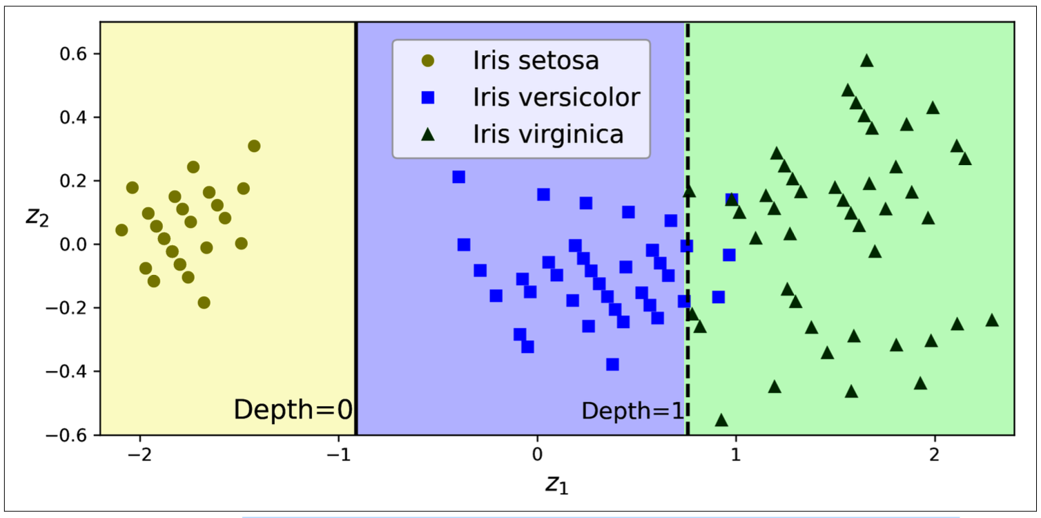
=> Solution: Scale data -> PCA: reduce dimensions but do not loss too much information, rotate data to reduce correlation between features, which often (not always) makes things easier for trees.
Compare to Figure fig-decision-tree, the scaled and PCA-rotated iris dataset is separated easier.
Figure 9.7: Scaled and PCA-rotated data
High variance: randomly select set of features to evaluate at each node, so that if we retrain model on the same dataset, it can behave really different => high variance, unstable
=> Solution: Ensemble methods (Random Forest, Boosting methods) averaging predictions over many trees.