11  Ensemble Learning

What would we do if we tried training multiple models but the results were not good enough? Let think about ensemble learning. Ensemble learning is a machine learning technique that combines the predictions of multiple weak learners to create a strong learner.

Ensemble learning offers several advantages:

• Improved Accuracy: Combining predictions from diverse models often leads to better overall performance compared to individual models.

• Reduced Overfitting: Ensemble methods trade higher bias for lower variance, in order to mitigate overfitting, especially when using techniques like bagging and proper hyperparameter tuning.

• Increased Robustness: Ensemble models are more resilient to noisy data and outliers.

• Enhanced Generalization: The diversity of models in an ensemble allows for better generalization to unseen data.

However, ensemble learning also comes with increased computational complexity and may require more careful tuning of hyperparameters. The choice of ensemble method depends on the characteristics of the data and the specific problem at hand.

Key ensemble learning techniques

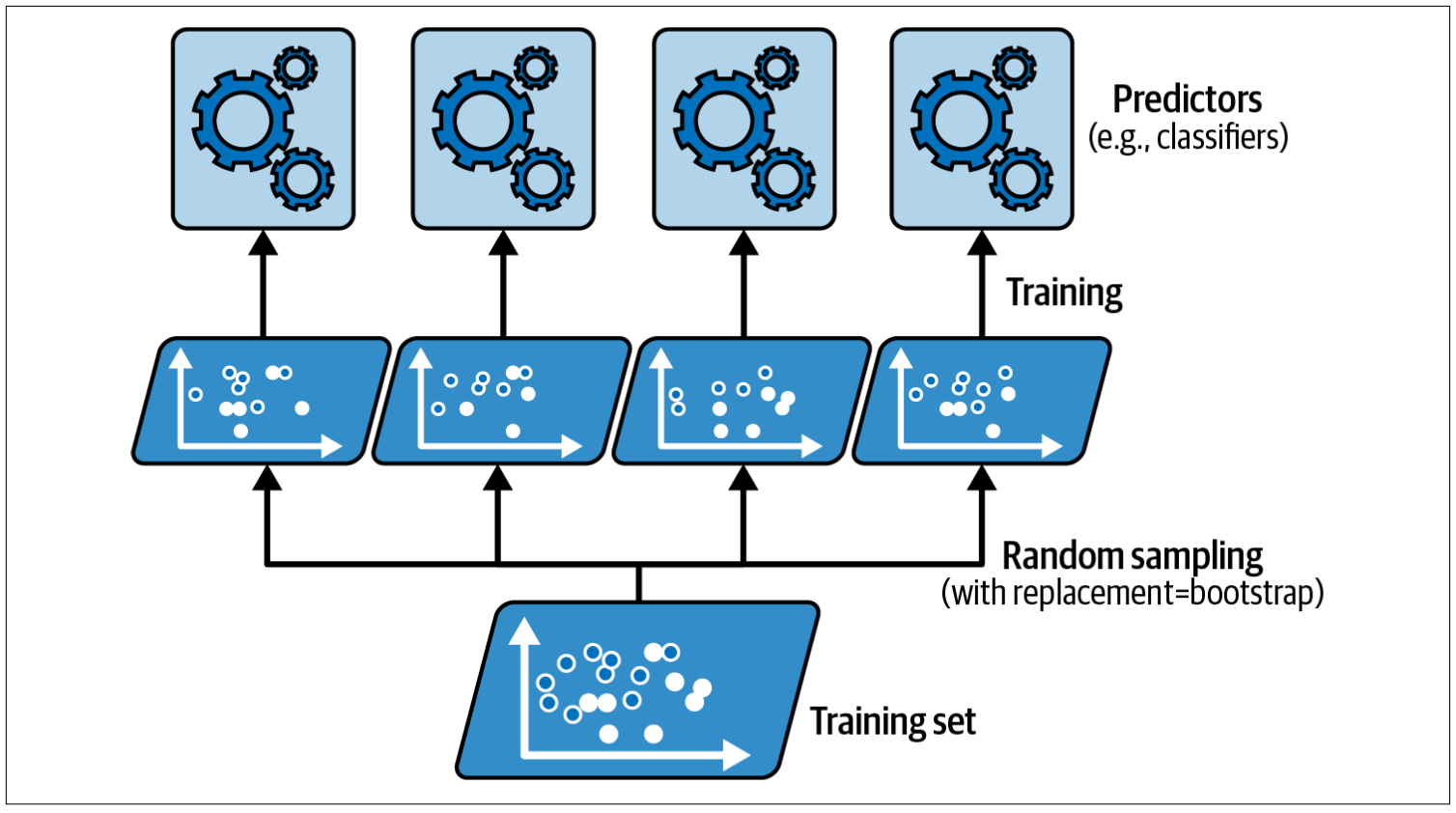
Bagging (Bootstrap Aggregating): Training multiple learner parallely on subset of dataset sampled with/without replacement (equally variables) using random subset of variables at each step of spliting internal node. Measure performance by ‘Out-Of-Bag Error’. Random Forests (ensemble of decision trees) are a notable example.

Boosting: Training multiple learner sequentially on full dataset, each subsequent model adjust the weights by correcting the errors of the previous ones (weighted variables). Popular algorithms using boosting include AdaBoost, Gradient Boosting (e.g., XGBoost, LightGBM), and CatBoost.

Stacking: Stacking combines predictions from multiple models by training a meta-model on their outputs. Base models act as input features for the meta-model, which learns to make a final prediction.

Random forests, AdaBoost, and GBRT are among the first models you should test for most machine learning tasks, and they particularly shine with heterogeneous tabular data. Moreover, as they require very little preprocessing, they’re great for getting a prototype up and running quickly. Lastly, ensemble methods like voting classifiers and stacking classifiers can help push your system’s performance to its limits.

Hyperparameters:

• Bagging methods: n_estimators, bootstrap, max_samples, bootstrap_features, max_features, oob_score.
• Decision tree: hyperparameters.
• Gradient Boosting: learning_rate, early_stopping, n_iter_no_change, tol, validation_fraction, subsample (like max_samples).

11.1 Bagging

11.1.1 Voting Classifier

The simpliest bagging algorithm with no boostrapping and only aggregating. It aggregates predictions by choosing most voted class (hard voting) or class with highest probability (soft voting).

In sklearn.ensemble.VotingClassifier, it performs hard voting by default.

from sklearn.datasets import make_moons
from sklearn.model_selection import train_test_split
from sklearn.linear_model import LogisticRegression
from sklearn.ensemble import VotingClassifier, RandomForestClassifier
from sklearn.svm import SVC

X, y = make_moons(n_samples=500, noise=0.30, random_state=42)
X_train, X_test, y_train, y_test = train_test_split(X, y, random_state=42)
voting_clf = VotingClassifier(
        estimators=[
            ('lr', LogisticRegression(random_state=42)),
            ('rf', RandomForestClassifier(random_state=42)),
            ('svc', SVC(random_state=42))
] )
voting_clf.fit(X_train, y_train)

print('Accuracy of individual predictor:')
for name,clf in voting_clf.named_estimators_.items():
    print(f'{name} = {clf.score(X_test,y_test)}')

print(f'Accuracy of ensemble: {voting_clf.score(X_test, y_test)}')

Accuracy of individual predictor:
lr = 0.864
rf = 0.896
svc = 0.896
Accuracy of ensemble: 0.912

Change to soft voting

voting_clf.voting = 'soft'
voting_clf.named_estimators['svc'].probability = True
voting_clf.fit(X_train, y_train)
voting_clf.score(X_test, y_test)

0.92

11.1.2 Bagging and Pasting

• Training multiple learner parallely => Scale very well.
• Sampling with replacement (Bagging); sampling without replacement (pasting).

Figure 11.1: Bagging and Pasting

• Sampling instances : max_samples indicates number/proportion of instances used to train model; bootstrap=True/False.
• Sampling features: max_features and bootstrap_features work the same.
  
  • Random patches: sampling instances and features
    
  • Random subspaces: sampling only features.
    
• The randomness trades a higher bias for lower variance.

from sklearn.ensemble import BaggingClassifier
from sklearn.tree import DecisionTreeClassifier

bagging_clf = BaggingClassifier(DecisionTreeClassifier(), n_estimators=500, max_samples=100, random_state=29)

bagging_clf.fit(X_train, y_train)
bagging_clf.score(X_train, y_train)

0.9413333333333334

Figure 11.2: Bagging decision trees

• Measure performance by Out-Of-Bag Error: set oob_score=True; the score made on the remaining not sampled instances.

bagging_clf = BaggingClassifier(DecisionTreeClassifier(), n_estimators=500, oob_score=True, max_samples=100, random_state=29)

bagging_clf.fit(X_train, y_train)
bagging_clf.oob_score_

0.9226666666666666

11.1.3 Random Forest

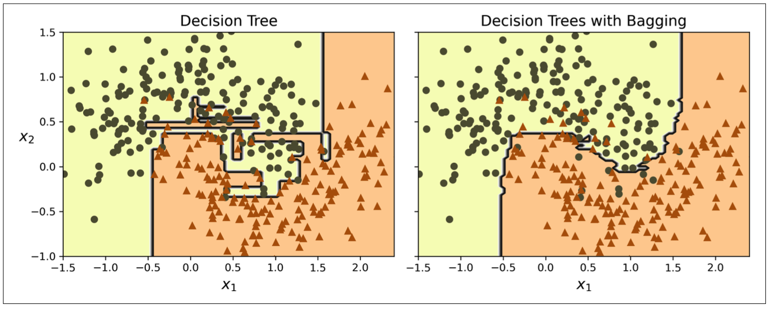
Random forest is ensemble of decision trees using bagging on full dataset. RandomForestClassifier has all the hyperparameters of DecisionTreeClassifier and BaggingClassifier to control ensemble.

from sklearn.ensemble import RandomForestClassifier

rf_clf = RandomForestClassifier(n_estimators=500, max_leaf_nodes=16, min_samples_leaf=10, random_state=29)
rf_clf.fit(X_train, y_train)
rf_clf.score(X_test, y_test)

0.92

Add more randomness:

• Decision tree: searching for the best possible thresholds of each feature.
• Extra-trees: search for best feature using random thresholds for each feature. Use RandomForestClassifier(splitter=“random”) or ExtraTreesClassifier.

bagging_clf = BaggingClassifier(DecisionTreeClassifier(splitter='random'), n_estimators=500, random_state=29)
bagging_clf.fit(X_train, y_train)
print(f'Random forest: {bagging_clf.score(X_test, y_test)}')

from sklearn.ensemble import ExtraTreesClassifier

extra_tree = ExtraTreesClassifier(n_estimators=500, random_state=29)
extra_tree.fit(X_train, y_train)
print(f'Extra trees: {extra_tree.score(X_test, y_test)}')

Random forest: 0.888

Extra trees: 0.88

11.1.4 Feature importance

Although we have state that bagging method treat all features equally, there is still a method to get the weighted average after training by look at the proportion of training samples used to reduce impurity. This can be used to perform features selection.

from sklearn.datasets import load_iris
iris = load_iris(as_frame=True)
rf_clf = RandomForestClassifier(n_estimators=500, random_state=42)
rf_clf.fit(iris.data, iris.target)

for score,feature in zip(rf_clf.feature_importances_, iris.data.columns):
    print(f'{feature}: {score:.3f}')

sepal length (cm): 0.112
sepal width (cm): 0.023
petal length (cm): 0.441
petal width (cm): 0.423

11.2 Boosting

We will talk about AdaBoost (adaptive boosting) and Gradient boosting.

11.2.1 AdaBoost

The algorithm work by training predictors sequentially. First it trains the base model and make predictions, then train the new pridictor weighting more on misclassified instances of the previous one, and so on. This is one of the most powerful model, and its main drawback is just do not scale really well.

Figure 11.3: AdaBoost

Fundamentals:

1. Initialize weights w(i) of each instance equal to 1/m

2. Train base predictor

3. Predict and get weighted error rate r(j) Weighted error rate of the j(th) predictor \[r_j = \sum_{i=1}^{m}w^{(i)}\;\;\;with\;yhat_{j}^{(i)}\;≠\;y^{(i)}\]

4. Compute predictor’s weight α(j). The more accurate the predictor, the higher its α(j)

\[α_j = ηlog(\frac{1-r_j}{r_j})\]

5. Update instances’s weights. This give more weights on misclassified instances.

\[ \begin{equation} \begin{split} w^{(i)} &= w^{(i)}\;\;\;\;\;\;\;\;\;\;\;\;\;\;if\;yhat_{j}^{(i)} = y^{(i)}\\ &=w^{(i)}exp(α_j)\;\;if\;yhat_{j}^{(i)} ≠ y^{(i)} \end{split} \end{equation} \]

6. Normalize all instances’s weights.

\[w^{(i)} = \frac{w^{(i)}}{\sum_{i=1}^{m}w^{(i)}}\]

7. Train new predictor using these weights
8. Stop training when number of predictors is reached, or when a perfect predictor is found.
9. Predict by majority vote.

from sklearn.ensemble import AdaBoostClassifier

ada_clf = AdaBoostClassifier(estimator=DecisionTreeClassifier(), learning_rate=0.001, n_estimators=100, random_state=29)

ada_clf.fit(X_train, y_train)
ada_clf.score(X_test, y_test)

0.824

11.2.2 Gradient Boosting

As same as AdaBoost, but instead of tweaking the instance weights, this method tries to fit the new predictor to the log loss (classification)/residual errors (regression) made by the previous predictor.

Regularization technique: shrinkage, adjust the learning rate.

Sampling instances: Stochastic Gradient Boosting; set subsample hyperparameter.

from sklearn.ensemble import GradientBoostingClassifier

gb_clf = GradientBoostingClassifier(n_estimators=50, max_depth=2, learning_rate=0.05, n_iter_no_change=10)
gb_clf.fit(X_train, y_train)
gb_clf.score(X_test, y_test)

0.912

11.2.3 Histogram-Based Gradient Boosting

Optimize for large dataset. It works by binning the input features, replacing them with integers, in which max_bins ≤ 255. It’s more faster but causes a precision loss => Risk of underfitting.

Learn more about XGBoost, CatBoost and LightGBM

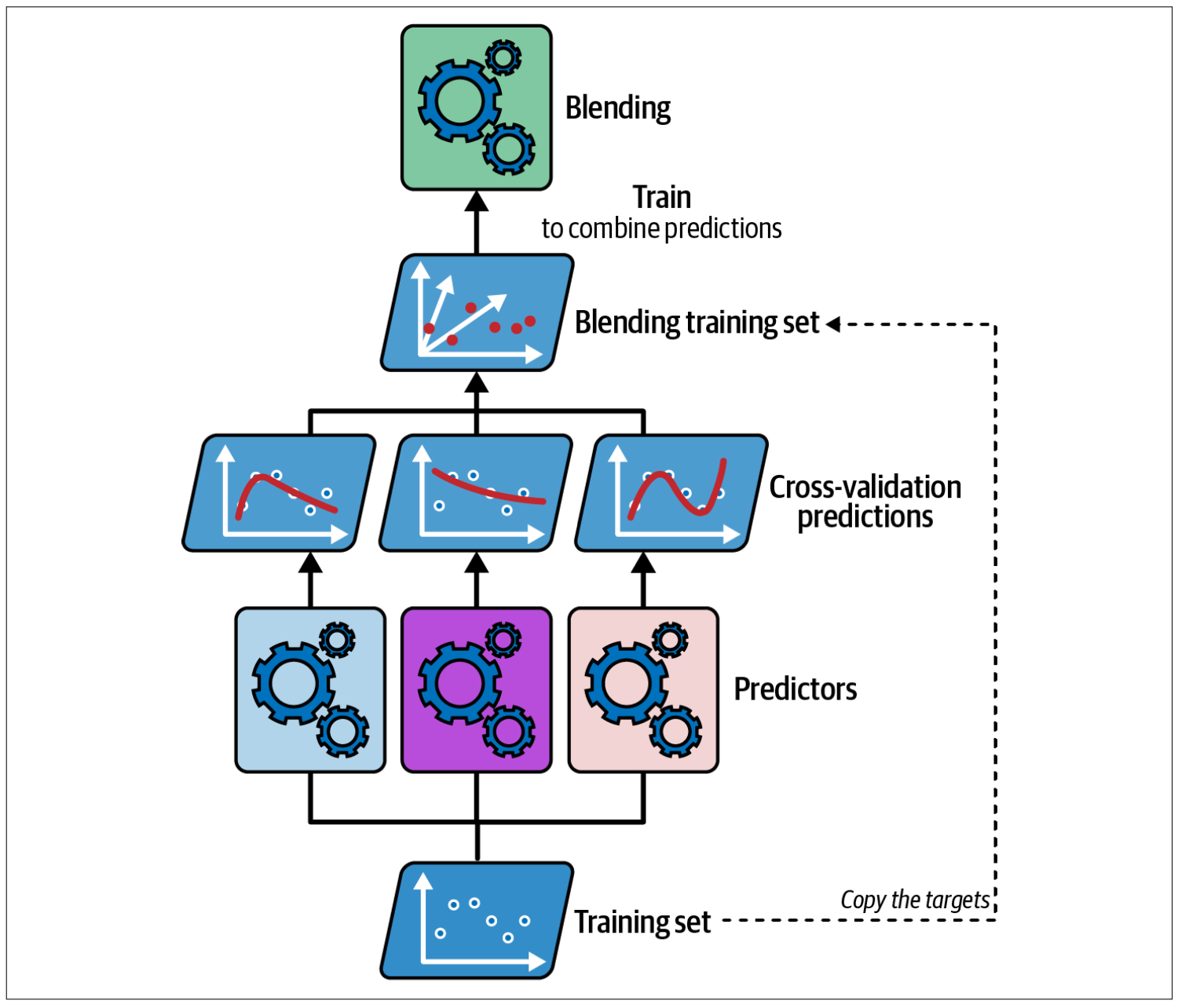
11.3 Stacking (Stacked Generalization)

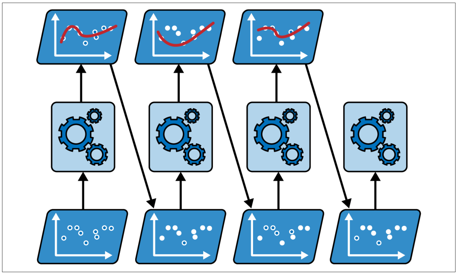
Stacking method works by training a model to aggregate the predictions instead of majority voting like bagging method. This model, also called blender or meta learner, uses the prediction of weak learners (out-of-sample) as input and makes final prediction.

Figure 11.4: Stacking method

from sklearn.ensemble import StackingClassifier
from sklearn.svm import LinearSVC

stacking_clf = StackingClassifier(
    estimators=[
        ('logis', LogisticRegression(random_state=29)),
        ('rf', RandomForestClassifier(random_state=29)),
        ('svc', LinearSVC(random_state=29))
    ],
    final_estimator=RandomForestClassifier(random_state=29),
    cv=5
)
stacking_clf.fit(X_train, y_train)
stacking_clf.score(X_test, y_test)

/usr/local/anaconda3/envs/dhuy/lib/python3.11/site-packages/sklearn/svm/_classes.py:32: FutureWarning:

The default value of `dual` will change from `True` to `'auto'` in 1.5. Set the value of `dual` explicitly to suppress the warning.

/usr/local/anaconda3/envs/dhuy/lib/python3.11/site-packages/sklearn/svm/_classes.py:32: FutureWarning:

The default value of `dual` will change from `True` to `'auto'` in 1.5. Set the value of `dual` explicitly to suppress the warning.

/usr/local/anaconda3/envs/dhuy/lib/python3.11/site-packages/sklearn/svm/_classes.py:32: FutureWarning:

The default value of `dual` will change from `True` to `'auto'` in 1.5. Set the value of `dual` explicitly to suppress the warning.

/usr/local/anaconda3/envs/dhuy/lib/python3.11/site-packages/sklearn/svm/_classes.py:32: FutureWarning:

The default value of `dual` will change from `True` to `'auto'` in 1.5. Set the value of `dual` explicitly to suppress the warning.

/usr/local/anaconda3/envs/dhuy/lib/python3.11/site-packages/sklearn/svm/_classes.py:32: FutureWarning:

The default value of `dual` will change from `True` to `'auto'` in 1.5. Set the value of `dual` explicitly to suppress the warning.

/usr/local/anaconda3/envs/dhuy/lib/python3.11/site-packages/sklearn/svm/_classes.py:32: FutureWarning:

The default value of `dual` will change from `True` to `'auto'` in 1.5. Set the value of `dual` explicitly to suppress the warning.

0.896

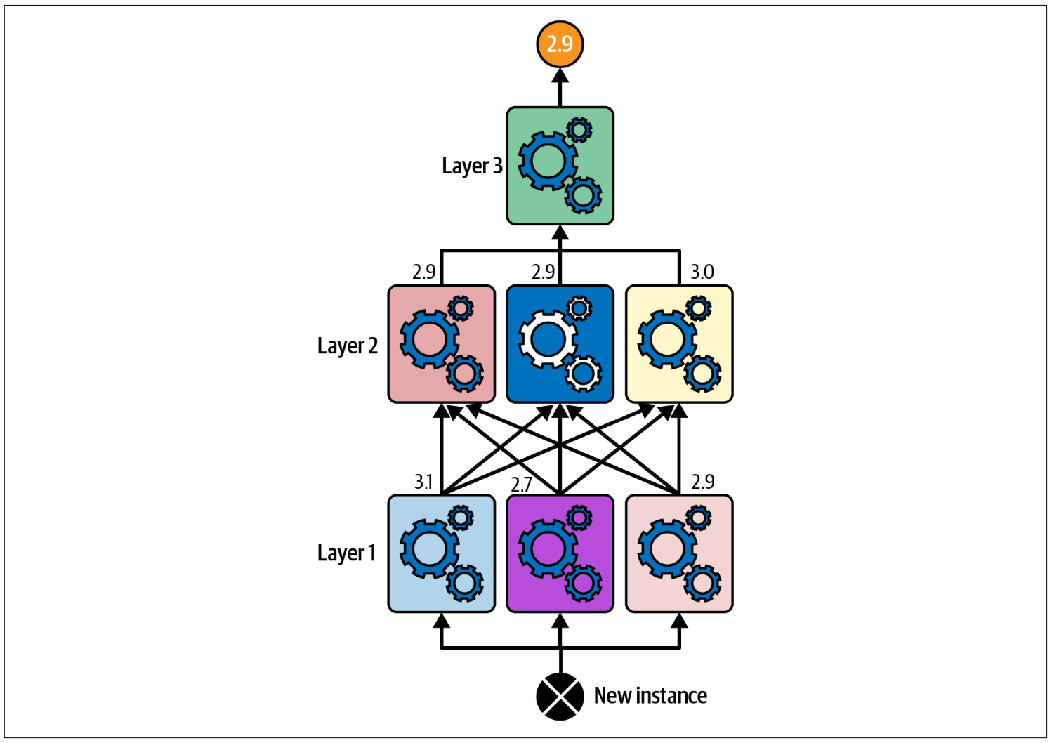
It can be created with layer of blenders such like this

Figure 11.5: Multilayer stacking

If you don’t provide a final estimator, StackingClassifier will use LogisticRegression and StackingRegressor will use RidgeCV.