7  Hands-on Classification

7.1 Describe the used dataset

• Name: MNIST
• Author: Yann LeCun, Corinna Cortes, Christopher J.C. Burges
• Content: 70,000 images of digits handwritten
• Source: MNIST Website

7.2 Get data

7.2.1 Download data

from sklearn.datasets import fetch_openml

mnist = fetch_openml('mnist_784', as_frame=False)       # as_frame=False: get data as Numpy Array instead of Pandas DataFrame
mnist.DESCR

/usr/local/anaconda3/envs/dhuy/lib/python3.11/site-packages/sklearn/datasets/_openml.py:1022: FutureWarning:

The default value of `parser` will change from `'liac-arff'` to `'auto'` in 1.4. You can set `parser='auto'` to silence this warning. Therefore, an `ImportError` will be raised from 1.4 if the dataset is dense and pandas is not installed. Note that the pandas parser may return different data types. See the Notes Section in fetch_openml's API doc for details.

"**Author**: Yann LeCun, Corinna Cortes, Christopher J.C. Burges  \n**Source**: [MNIST Website](http://yann.lecun.com/exdb/mnist/) - Date unknown  \n**Please cite**:  \n\nThe MNIST database of handwritten digits with 784 features, raw data available at: http://yann.lecun.com/exdb/mnist/. It can be split in a training set of the first 60,000 examples, and a test set of 10,000 examples  \n\nIt is a subset of a larger set available from NIST. The digits have been size-normalized and centered in a fixed-size image. It is a good database for people who want to try learning techniques and pattern recognition methods on real-world data while spending minimal efforts on preprocessing and formatting. The original black and white (bilevel) images from NIST were size normalized to fit in a 20x20 pixel box while preserving their aspect ratio. The resulting images contain grey levels as a result of the anti-aliasing technique used by the normalization algorithm. the images were centered in a 28x28 image by computing the center of mass of the pixels, and translating the image so as to position this point at the center of the 28x28 field.  \n\nWith some classification methods (particularly template-based methods, such as SVM and K-nearest neighbors), the error rate improves when the digits are centered by bounding box rather than center of mass. If you do this kind of pre-processing, you should report it in your publications. The MNIST database was constructed from NIST's NIST originally designated SD-3 as their training set and SD-1 as their test set. However, SD-3 is much cleaner and easier to recognize than SD-1. The reason for this can be found on the fact that SD-3 was collected among Census Bureau employees, while SD-1 was collected among high-school students. Drawing sensible conclusions from learning experiments requires that the result be independent of the choice of training set and test among the complete set of samples. Therefore it was necessary to build a new database by mixing NIST's datasets.  \n\nThe MNIST training set is composed of 30,000 patterns from SD-3 and 30,000 patterns from SD-1. Our test set was composed of 5,000 patterns from SD-3 and 5,000 patterns from SD-1. The 60,000 pattern training set contained examples from approximately 250 writers. We made sure that the sets of writers of the training set and test set were disjoint. SD-1 contains 58,527 digit images written by 500 different writers. In contrast to SD-3, where blocks of data from each writer appeared in sequence, the data in SD-1 is scrambled. Writer identities for SD-1 is available and we used this information to unscramble the writers. We then split SD-1 in two: characters written by the first 250 writers went into our new training set. The remaining 250 writers were placed in our test set. Thus we had two sets with nearly 30,000 examples each. The new training set was completed with enough examples from SD-3, starting at pattern # 0, to make a full set of 60,000 training patterns. Similarly, the new test set was completed with SD-3 examples starting at pattern # 35,000 to make a full set with 60,000 test patterns. Only a subset of 10,000 test images (5,000 from SD-1 and 5,000 from SD-3) is available on this site. The full 60,000 sample training set is available.\n\nDownloaded from openml.org."

7.2.2 Quick Look

## Size of dataset

X,y = mnist.data, mnist.target
print(X.shape, y.shape)

(70000, 784) (70000,)

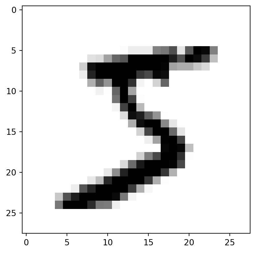
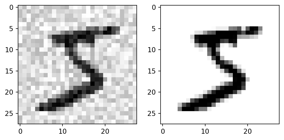
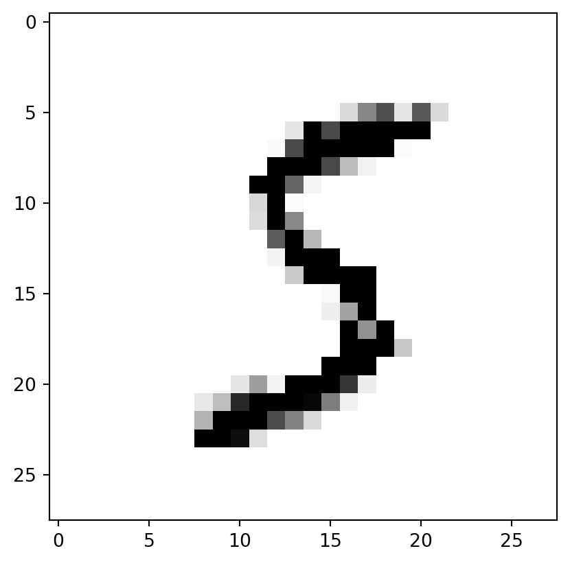
## Quick look

import matplotlib.pyplot as plt

def plot_digit(data):
    image = data.reshape(28,28)
    plt.imshow(image, cmap='binary')   # binary: grayscale color map from 0 (white) to 255 (black)
    
some_digit = X[0]    # Look at first digit
plot_digit(some_digit)
plt.show()

7.2.3 Create train, test set

## Split dataset into train set and test set as its describe (train: first 60000 images, test: last 10000 images)

X_train, X_test, y_train, y_test = X[:60000], X[60000:], y[:60000], y[60000:]
print(X_train.shape)

(60000, 784)

7.3 Create a Binary Classfier(5 or non-5)

## Target labels

y_train_5 = (y_train == '5')
y_test_5 = (y_test == '5')

7.3.1 Stochastic Gradient Descent

7.3.1.1 Train model

from sklearn.linear_model import SGDClassifier

sgd_clf = SGDClassifier(random_state=42)
sgd_clf.fit(X_train, y_train_5)

sgd_clf.predict([some_digit])

array([ True])

7.3.1.2 Evaluate model

Metrics:
- Accuracy
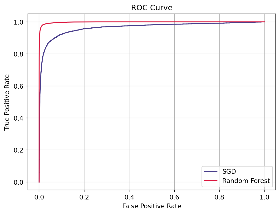
- Confusion matrix: Precision, Recall (TPR), FPR, ROC, ROC AUC
- Plot: Precision-Recall Curve, ROC Curve
Use case:
- Precision-Recall Curve: aim to care more about false positives than the false negatives
- Otherwise: ROC Curve

Accuracy

from sklearn.model_selection import cross_val_score

cross_val_score(sgd_clf, X_train, y_train_5, cv=3, scoring='accuracy')

array([0.95035, 0.96035, 0.9604 ])

The accuracy scores are pretty good, but it may be due to the class imbalance. Let take a look at a Dummy Model which always classify as the most frequent class

## Dummy classifier

from sklearn.dummy import DummyClassifier
from sklearn.model_selection import cross_val_score

dummy_model = DummyClassifier(random_state=248)
cross_val_score(dummy_model, X_train, y_train_5, cv=3, scoring='accuracy')

array([0.90965, 0.90965, 0.90965])

The accuracy scores are over 90% because there’s only about 10% of training set are 5 digit
=> With class imbalance, accuracy score is not a useful metric
=> We will use other metrics such as Precision, Recall, ROC Curve, AUC

Confusion Matrix

from sklearn.model_selection import cross_val_predict
from sklearn.metrics import confusion_matrix

y_train_pred = cross_val_predict(sgd_clf, X_train, y_train_5, cv=3)
confusion_matrix(y_train_5, y_train_pred)

array([[53892,   687],
       [ 1891,  3530]])

## Precision and Recall

from sklearn.metrics import precision_score, recall_score

print(f'Precision scores: {precision_score(y_train_5, y_train_pred):.4f}')
print(f'Recall scores: {recall_score(y_train_5, y_train_pred):.4f}')

Precision scores: 0.8371
Recall scores: 0.6512

## F1-score

from sklearn.metrics import f1_score

print(f'F1-score: {f1_score(y_train_5, y_train_pred):.4f}')

F1-score: 0.7325

Precision-Recall Trade-off

• Compute the scores of all instances in the training using decision_function
• Change the threshold to see the difference

y_score = sgd_clf.decision_function([some_digit])

threshold = [0, 1000, 3000]
for thr in threshold:
    print(f'With threshold of {thr:4d}: predicted value is {y_score>thr}')

With threshold of    0: predicted value is [ True]
With threshold of 1000: predicted value is [ True]
With threshold of 3000: predicted value is [False]

How to choose the suitable threshold?

• Use Precision-Recall Curve
• precision_recall_curve: require scores computed from decision_function or probabilities from predict_proba

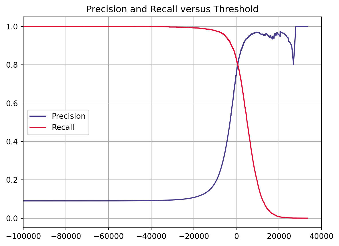
## Precision-Recall Curve


### Compute scores by decision_function

y_scores = cross_val_predict(sgd_clf, X_train, y_train_5, method='decision_function')

### Plot Precision-Recall Curve vs Threshold

from sklearn.metrics import precision_recall_curve

precisions, recalls, thresholds = precision_recall_curve(y_train_5, y_scores)

plt.plot(thresholds, precisions[:-1], label='Precision', color='darkslateblue')
plt.plot(thresholds, recalls[:-1], label='Recall', color='crimson')
plt.grid()
plt.legend(loc='center left')
plt.xlim([-100000,40000])
plt.title('Precision and Recall versus Threshold')
plt.show()

The higher Precision, the lower Recall and vice versa

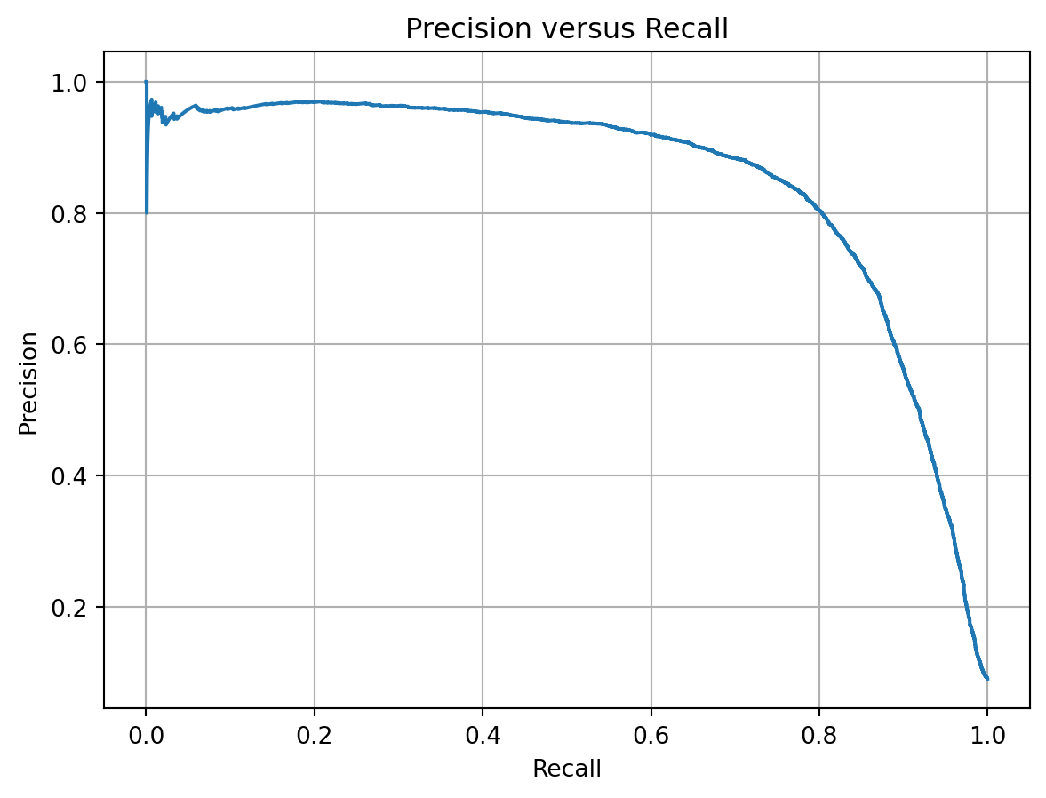
## Plot Precision versus Recall

plt.plot(recalls, precisions)
plt.title('Precision versus Recall')
plt.xlabel('Recall')
plt.ylabel('Precision')
plt.grid()

plt.show()

Depend on your project, you would trade between precision and recall

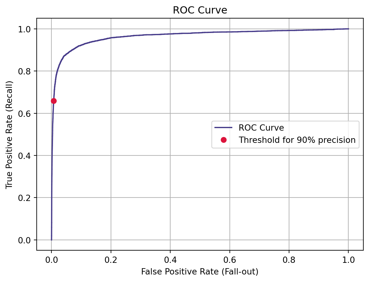
## Find Threshold of over 0.90 Precision

idx_90_precision = (precisions >= 0.90).argmax()
threshold_90_precision = thresholds[idx_90_precision]
threshold_90_precision

3045.9258227053647

y_train_90_precision = (y_scores > threshold_90_precision)

from sklearn.metrics import accuracy_score
print(f'Accuracy score: {accuracy_score(y_train_5, y_train_90_precision):.4f}')
print(f'Precision score: {precision_score(y_train_5, y_train_90_precision):.4f}')
print(f'Recall score: {recall_score(y_train_5, y_train_90_precision):.4f}')
print(f'F1 score: {f1_score(y_train_5, y_train_90_precision):.4f}')

Accuracy score: 0.9626
Precision score: 0.9002
Recall score: 0.6587
F1 score: 0.7608

## ROC AUC

from sklearn.metrics import roc_auc_score, roc_curve

print(f'AUC score: {roc_auc_score(y_train_5, y_scores):.4f}')       

AUC score: 0.9648

## ROC Curve

fpr, tpr, thresholds = roc_curve(y_train_5, y_scores)
idx_threshold_90_precision = (thresholds<=threshold_90_precision).argmax()      # thresholds listed decreasing => use (<=)
fpr_90, tpr_90 = fpr[idx_threshold_90_precision], tpr[idx_threshold_90_precision]

plt.plot(fpr, tpr, label='ROC Curve', color='darkslateblue')
plt.plot([fpr_90], [tpr_90], 'o', label='Threshold for 90% precision', color='crimson')
plt.title('ROC Curve')
plt.xlabel('False Positive Rate (Fall-out)')
plt.ylabel('True Positive Rate (Recall)')
plt.legend(loc='center right')
plt.grid()

plt.show()

Another trade-off: The higher TPR, the lower FPR and vice versa

7.3.2 Logistic Regression

from sklearn.linear_model import LogisticRegression

logistic = LogisticRegression(random_state=29)

y_pred_logis = cross_val_predict(logistic, X_train, y_train_5, cv=3, method='predict_proba')[:,1]

/usr/local/anaconda3/envs/dhuy/lib/python3.11/site-packages/sklearn/linear_model/_logistic.py:460: ConvergenceWarning:

lbfgs failed to converge (status=1):
STOP: TOTAL NO. of ITERATIONS REACHED LIMIT.

Increase the number of iterations (max_iter) or scale the data as shown in:
    https://scikit-learn.org/stable/modules/preprocessing.html
Please also refer to the documentation for alternative solver options:
    https://scikit-learn.org/stable/modules/linear_model.html#logistic-regression

/usr/local/anaconda3/envs/dhuy/lib/python3.11/site-packages/sklearn/linear_model/_logistic.py:460: ConvergenceWarning:

lbfgs failed to converge (status=1):
STOP: TOTAL NO. of ITERATIONS REACHED LIMIT.

Increase the number of iterations (max_iter) or scale the data as shown in:
    https://scikit-learn.org/stable/modules/preprocessing.html
Please also refer to the documentation for alternative solver options:
    https://scikit-learn.org/stable/modules/linear_model.html#logistic-regression

/usr/local/anaconda3/envs/dhuy/lib/python3.11/site-packages/sklearn/linear_model/_logistic.py:460: ConvergenceWarning:

lbfgs failed to converge (status=1):
STOP: TOTAL NO. of ITERATIONS REACHED LIMIT.

Increase the number of iterations (max_iter) or scale the data as shown in:
    https://scikit-learn.org/stable/modules/preprocessing.html
Please also refer to the documentation for alternative solver options:
    https://scikit-learn.org/stable/modules/linear_model.html#logistic-regression

## Measure performance

threshold = 0.5
f1_logis = f1_score(y_train_5, y_pred_logis>=threshold)
auc_logis = roc_auc_score(y_train_5, y_pred_logis>=threshold)

print(f'F1 score Random Forest: {f1_logis:.4f}')
print(f'AUC Random Forest: {auc_logis:.4f}')

F1 score Random Forest: 0.8487
AUC Random Forest: 0.9004

7.3.3 Random Forest

from sklearn.ensemble import RandomForestClassifier

rf_clf = RandomForestClassifier(random_state=42)

y_train_pred_rf = cross_val_predict(rf_clf, X_train, y_train_5, cv=3, method='predict_proba')[:,1]

## Measure performance

threshold = 0.5
f1_rf = f1_score(y_train_5, y_train_pred_rf>=threshold)
auc_rf = roc_auc_score(y_train_5, y_train_pred_rf>=threshold)

print(f'F1 score Random Forest: {f1_rf:.4f}')
print(f'AUC Random Forest: {auc_rf:.4f}')

F1 score Random Forest: 0.9275
AUC Random Forest: 0.9358

## PR Curve

precisions_rf, recalls_rf, thresholds_rf = precision_recall_curve(y_train_5, y_train_pred_rf)

plt.plot(recalls, precisions, "-", label='SGD')
plt.plot(recalls_rf, precisions_rf, label='Random Forest')
plt.title('Precision versus Recall')
plt.xlabel('Recall')
plt.ylabel('Precision')
plt.legend()
plt.grid()

plt.show()

## ROC Curve

fpr_rf, tpr_rf, thresholds = roc_curve(y_train_5, y_train_pred_rf)

plt.plot(fpr, tpr, label='SGD', color='darkslateblue')
plt.plot(fpr_rf, tpr_rf, label='Random Forest', color='crimson')
plt.title('ROC Curve')
plt.xlabel('False Positive Rate')
plt.ylabel('True Positive Rate')
plt.legend()
plt.grid()

plt.show()

7.4 Multiclass Classification

• LogisticRegression, RandomForestClassifier, GaussianNB: natively handle Multiclass Classification

• SGDClassifier and SVC: strictly binary classifiers

  • ovo: one versus one strategy, preferred with scale poorly algorithms (i.e. SVC)
  • ovr: one versus rest strategy, preferred for almost algorithms

7.4.1 SVC

7.4.1.1 Default: ovo strategy

from sklearn.svm import SVC

svc_clf = SVC(random_state=42)
svc_clf.fit(X_train[:1000], y_train[:1000])
svc_clf.predict([some_digit])

array(['5'], dtype=object)

## Scores from decision_function

some_digit_svc = svc_clf.decision_function([some_digit])
some_digit_svc.round(4)

array([[ 1.7583,  2.7496,  6.1381,  8.2854, -0.2873,  9.3012,  0.7423,
         3.7926,  7.2085,  4.8576]])

## Class of highest score

idx_svc = some_digit_svc.argmax()
idx_svc

5

## Classes of prediction
svc_clf.classes_[idx_svc]

'5'

7.4.1.2 Force: ovr strategy

## Train model

from sklearn.multiclass import OneVsRestClassifier

ovr_svc_clf = OneVsRestClassifier(SVC(random_state=42))
ovr_svc_clf.fit(X[:1000], y_train[:1000])
ovr_svc_clf.predict([some_digit])

array(['5'], dtype='<U1')

## Compute scores

some_digit_ovr_svc = ovr_svc_clf.decision_function([some_digit])
some_digit_ovr_svc.round(4)

array([[-1.3439, -1.5195, -1.221 , -0.9294, -2.0057,  0.6077, -1.6226,
        -0.9998, -1.2764, -1.7031]])

## Class of hishest score

some_digit_ovr_svc.argmax()

5

## Extract classes

ovr_svc_clf.classes_

array(['0', '1', '2', '3', '4', '5', '6', '7', '8', '9'], dtype='<U1')

7.4.2 SGD

## Train model

from sklearn.linear_model import SGDClassifier

sgd_clf = SGDClassifier(random_state=42)
sgd_clf.fit(X_train, y_train)
sgd_clf.predict([some_digit])

array(['3'], dtype='<U1')

That’s incorrect. As we can see,The Classifier is not very confident about its prediction.

## Compute scores

sgd_clf.decision_function([some_digit])

array([[-31893.03095419, -34419.69069632,  -9530.63950739,
          1823.73154031, -22320.14822878,  -1385.80478895,
        -26188.91070951, -16147.51323997,  -4604.35491274,
        -12050.767298  ]])

We will use cross validation to evaluate our model

cross_val_score(sgd_clf, X_train, y_train, cv=3, scoring='accuracy')

array([0.87365, 0.85835, 0.8689 ])

We can scale the data to get better result

from sklearn.preprocessing import StandardScaler

scaler = StandardScaler()
X_train_scaled = scaler.fit_transform(X_train.astype('float64'))
cross_val_score(sgd_clf, X_train_scaled, y_train, cv=3, scoring='accuracy')

array([0.8983, 0.891 , 0.9018])

Let’s look at the confusion matrix of our prediction

## Predict using cross_val_predict

from sklearn.metrics import ConfusionMatrixDisplay

y_train_pred = cross_val_predict(sgd_clf, X_train_scaled, y_train, cv=3)

Confusion matrix with (right) and without (left) normalization.

fig,ax = plt.subplots(1,2,figsize=(9, 4))

ConfusionMatrixDisplay.from_predictions(y_train, y_train_pred, ax=ax[0])
ax[0].set_title("Confusion matrix")
ConfusionMatrixDisplay.from_predictions(y_train, y_train_pred, ax=ax[1], normalize='true', values_format='.0%')
ax[1].set_title("CM normalized by row")

plt.show()

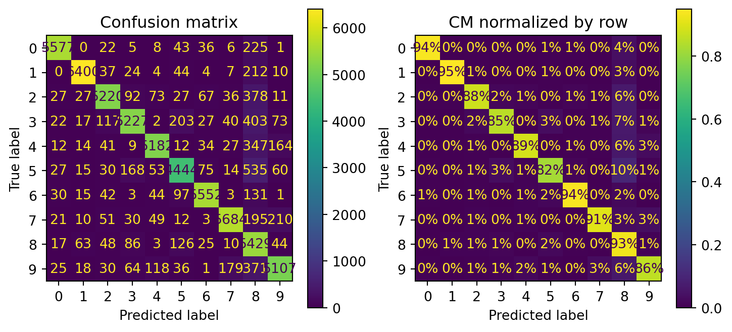
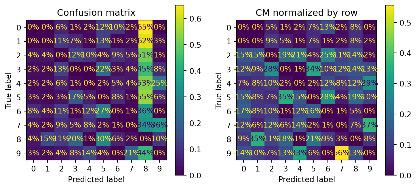
In row #5 and column #8 on the left plot, it’s means 10% of true 5s is misclassified as 8s. Kinda hard to see the errors made by model. Therefore, we will put 0 weight on correct prediction (error plot).

Confustion matrix with error normalized by row (left) and by column (right) (normalize=[‘true’,‘pred’])

fig,ax = plt.subplots(1,2,figsize=(9, 4))

sample_weight = (y_train != y_train_pred)

ConfusionMatrixDisplay.from_predictions(y_train, y_train_pred, ax=ax[0],sample_weight=sample_weight, normalize='true', values_format='.0%')
ax[0].set_title("Confusion matrix")
ConfusionMatrixDisplay.from_predictions(y_train, y_train_pred, ax=ax[1],sample_weight=sample_weight, normalize='pred', values_format='.0%')
ax[1].set_title("CM normalized by row")

plt.show()

In row #5 and column #8 on the left plot, it’s means 55% of errors made on true 5s is misclassified as 8s.

In row #5 and column #8 on the right plot, it’s means 19% of misclassified 8s are actually 5s.

Analyzing the made errors can help us gain insights and why the classifier failing

7.5 Multilabel Classification

Output is multilabel for each instances. For example, we will classify whether the digit is large (>7) and is odd

7.5.1 K Nearest Neighbors

## Train model

import numpy as np
from sklearn.neighbors import KNeighborsClassifier

y_train_large = (y_train >= '7')
y_train_odd = (y_train.astype('int8') % 2 == 1)
y_train_multilabel = np.c_[y_train_large, y_train_odd]

knn = KNeighborsClassifier()
knn.fit(X_train_scaled, y_train_multilabel)
knn.predict([some_digit])

array([[False,  True]])

Compute average F1 score across all labels (equally important)

## Evaluate model

y_train_pred_knn = cross_val_predict(knn, X_train_scaled, y_train, cv=3)
f1_score(y_train, y_train_pred_knn, average='macro')

0.9396793112547043

Another approach is to give each label a weight equal to its number of instances

f1_score(y_train, y_train_pred_knn, average='weighted')

0.940171964265114

7.5.2 SVC

• SVC does not natively support multilabel classification. Therefore, there are 2 strategies:

1. Train one model per label. It turns out that it’s hard to capture the dependencies between labels
2. Train models sequentially (ChainClassifier): using input features and all predictions of previous models in the chain

from sklearn.multioutput import ClassifierChain

chain_clf = ClassifierChain(SVC(), cv=3, random_state=42)
chain_clf.fit(X_train_scaled[:2000], y_train_multilabel[:2000])
chain_clf.predict([some_digit])

array([[0., 1.]])

7.6 Multioutput Classification

• Multiclass-multilabel classification
• For example, we will build a model that removes noise from an digit image
• Output is a clean image 28x28: multilabel (one label per pixel) and multiclass (pixel intensity range from 0-255 per label)

## Create a noisy train set

np.random.seed(42)

noise = np.random.randint(0,100,(len(X_train), 28*28))
X_train_noise = X_train + noise
y_train_noise = X_train

noise = np.random.randint(0,100,(len(X_test), 28*28))
X_test_noise = X_test + noise
y_test_noise = X_test

Let’s look at sample images

plt.subplot(1,2,1)
plot_digit(X_train_noise[0])
plt.subplot(1,2,2)
plot_digit(y_train_noise[0])

plt.show()

knn.fit(X_train_noise, y_train_noise)
y_pred_noise = knn.predict([X_train_noise[0]])
plot_digit(y_pred_noise)